This is the final part of my SAP NetWeaver 7.0, Basic Performance Tuning Guide.
You may wish to review
Part I,
Part II or Part
III.
In this part I will focus on the use of ABAP Runtime Analysis to check performance of ABAP programs/reports. This will help you locate areas of ABAP that are eating up valuable response time.
Execute transaction SE30.
Enter the transaction (or program or function module) that you wish to analyse:

Edit the “Measurement Restrictions” variant to either create your own, or simply adjust the DEFAULT.
This will allow us to display additional information which can be very useful when trying to determine performance problems.

Tick the “DB-level ops” option on the Statements tab:

On the Duration/Type tab, select “None” for Aggregation and tick “With memory use”:

The transaction or program you entered will be run, but you should see a prompt at the bottom of the screen telling you that the measurement process has started:

Perform the actions you need in the transaction/program.
Once you have finished, simply click Back (exit from the transaction) to the SE30 main screen:

The SE30 screen will display a prompt showing the analysis has finished:

The trace data is stored in a file on the SAP instance server.
This can be seen by clicking the “File Info…” button:

You can see the file name and path:

If you need to load the trace data again for analysis, you can simply click the “Other File…” button on the main screen.
It’s also possible to transfer the analysis files via RFC to another SAP system from the “Other File…” sub-screens.
This is very useful if you want to compare performance between two systems.
NOTE: The performance data files are only retained on the server for eight days. I haven’t found a way of extending this.
Let’s analyse the stats.
Click the Evaluate button:

You will see a basic breakdown of the transaction runtime performance analysis in histogram form.
The three different areas are shown (ABAP, Database and System) against time (as a percentage):

More details on this screen can be found here: https://help.sap.com/saphelp_nw70/helpdata/en/c6/617d27e68c11d2b2ab080009b43351/content.htm
The values shown correlate to the response times measured in the single record statistics plus the time required for analysis.
Note that DATABASE time above, also includes the time the system takes to open and close cursors etc, not just the SQL runtime.
For reference, the STAD output for the same operation (notice the slightly lower DB req time):

The most interesting buttons at the top of the SE30 screen are “Hit List”, “Table Hit List” and “Call hierarchy”.
Click the Hit List button:

The Hit List will be displayed in descending order (gross time):
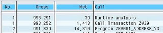
The columns are defined as follows:
“No.” – Shows the number of times a call was made.
If a “SELECT” is performed in a loop, then this will show the number of times the call was made in total in the loop.
“Gross” – Total execution time in microseconds (running bottom to top of the hit list).
“Net” – The time in microseconds for the specific call(s)
“Call” – The program component that was being executed.
“In program” – The main program of the component.
“Type” – The type of call (DB, System, Non-system).
SAP says here https://help.sap.com/saphelp_nw70/helpdata/en/c6/617d27e68c11d2b2ab080009b43351/content.htm:
“Gross time
The total time required for a call. This includes the runtime of all modularization units and ABAP statements called by the subject.
Net time
The net time is the gross time less the time required for modularization units (MODULE, PERFORM, CALL FUNCTION, CALL SCREEN, CALL TRANSACTION, CALL METHOD, CALL DIALOG, SUBMIT), and for the ABAP statements listed separately. For statements such as APPEND, the gross time is the same as the net time.“
In this view, you are looking for records in the list with the larger “Net” value.
This indicates that a large amount of overall time was spent in the call/program listed.
If the Gross and Net time fields do not hold the same value for a record, then double clicking the record will display the sub-components and switch to the hierarchy view:
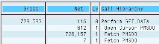
At any time, you can single click a record, then jump to the ABAP source by clicking the “Display Source Code” button:


NOTE: I always recommend you enable the “New” ABAP editor. It gives you visibility of line numbers and highlights the results of text “Find” operations so you can see what’s been found.
Back on the main analysis screen, select the “Table Hit List” button:

The list of tables used in the execution of the transaction/program are displayed in descending order of runtime:

The #Acces column, displays the number of times the table was accessed (read/write) and corresponds to any loops you may have seen in the “Hit List” screen No. column.
The Class column shows TRANSP (Transparent Table), VIEW or POOL (cluster table).
Double click a table to display the call points, from which you can jump to the ABAP source.
Finally, from the main analysis screen, click the “Call hierarchy” button:

The Hit List that you have already seen, will now be displayed in a hierarchy with sub-calls indented under the parent call:
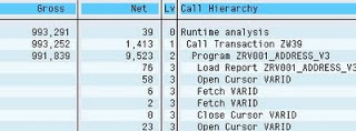
The only real difference between this view and the Hit List table view, is the indenting.
You can still double click to display the execution time overview for that sub-call, or use the “Display Source Code” button to jump to the ABAP source.
In my example screen shots, you will have seen that the PMSDO fetch is taking a large amount of the response time.
I was able to find that this operation was inside the GET_DATA function and check the ABAP code.
The main thing you are looking for in poor performing ABAP code, is where does the execution time get eaten up. As a side note, you may also check the amount of memory used if you are looking to resolve TSV PAGE ALLOC errors.
Try sorting the Hit List by “Net Time” to find the individual components with the highest net execution time.
Check if the operation is a database related call or not. You can then use Part III to trace this further with an SQL trace.
Check the number of loop iterations (The “No.” column) in the “Hit List”. Are you performing an expensive routine too many times in a loop?
Validate that the code is not doing too much work using iTabs, when some of the work could be done in the database.
The database is the ultimate place to do sorting, grouping and record elimination.
Don’t pull back more records than you need, only to loop through an iTab in ABAP and remove them, it’s more expensive.
That’s it for now. Thanks for reading.
