This blog contains experience gained over the years of implementing (and de-implementing) large scale IT applications/software.

Basic Performance Tuning Guide – SAP NetWeaver 7.0 – Part II – Reading Single Record Statistics

This is Part II. You may like to see Part I.

In Part I, we showed you how to trace an ABAP program using STAD to show the single record statistics of the response times for a transaction/program.
In this part, we will go through and decipher the statistics to help you decide where the problem may lie in your slow performing program.

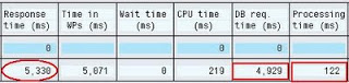
Following Part I, we saw the STAD screen output.  Below is a snapshot of the right hand side of the screen showing the “standard” view fields:
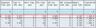
STAD output fields

The “Response time (ms)” field shows the total response time for the dialog step (or summary of steps if you have chosen not to expand the left tree).

As a reminder, SAP says (https://help.sap.com/saphelp_nw70ehp1/helpdata/en/21/2c8f38c7215428e10000009b38f8cf/content.htm
):
Response time = wait time + execution time
where: execution time =
Generation time during the run
+ Load time for programs, screens, and graphical user interfaces
+ Roll times for rolling in the work data
+ ABAP processing time
+ Database time
+ Enqueue time for logical SAP lock processes
+ CPIC/RFC time
+ Roll wait time (excluding task types RFC/CPIC/ALE).

So if we take a look at our initial screen of values, the example below shows that the “DB req time (ms)” is one of the larger values (4929):
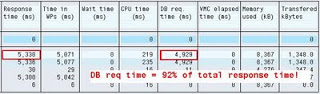
SAP STAD DB request time of response time

The total database request time (time taken for database work to be done for this step) is more than 92% of the total response time for the step.
If the database time IS NOT a significant percentage of total response time, then you should check the other parts that make up the total response time, for clues.

At this point, it’s better to change the screen columns so that you can see all the timings.
The best view is the “Time Analysis” view.  Switch views by clicking the “Sel. fields” button:

STAD select fields

Click “Time Analysis“:

STAD time analysis

You will now see more timing fields

STAD timing fields, response time

The fields highlighted are responsible for the total response time calculation.

In our example, TOTAL RESPONSE TIME = Wait Time + DB Req Time + Processing Time + Load Time + Generating Time + Roll In Time + Roll Wait Time + Enqueue Time.
=> 5330 = 0 + 4929 + 122 + 17 + 0 + 262 + 0
(5330 / 1000 = 5.3 seconds total response time)

You should check each of the fields, looking for disproportionate response times.

The “Wait time (ms)” indicates the amount of time the dialog step was waiting to be processed by a dialog work process.  High values indicate that the overall system performance is degraded.  Maybe a lack of memory, CPU or I/O performance at the O/S layer could be causing issues.  Check the dispatcher queue.

The “Time in WPs (ms)” indicates the time that the dialog step was being actively serviced by a work process and not by any other type of process (BTC, UPD, UPD2 etc). Check “SM51 -> Goto -> Server Name -> Information -> Queue Information” and SM66 to see how busy the system is.

The “Processing time (ms)” indicates the amount of time the individual components spent processing (working) and not idle or sleeping or waiting.  Check SM50 and SM66 to see how busy the system is.
Use ST06 (O/S monitor) to check CPU usage and system load.

The “Load time (ms)” indicates the amount of time taken to load the program code into memory buffers.
A problem here could indicate the program buffer is not large enough (see ST02).  You should check the CPU time if the load time value is large.

Values for “Generating time (ms)” show the time spent compiling the ABAP source code.  You will see a value here if the code has not already been compiled through SGEN.  Any large values here for programs already generated could mean a problem in the database with the code storage tables.

Large values for “Roll (i+w) time (ms)” indicates that the Roll-In and Roll-Wait times are being affected.
Roll-In is the process of moving the users session context into the work process so that it can be used to execute the dialog step.  High values could indicate that the roll buffer is too small (see ST02) or that the user has a very large set of roles and profiles and is consuming too much memory.

Values for “Enqueue time (ms)” show the time waited for a logical database lock to be performed.
A high value here could indicate excessive contention (someone else doing the same work) in the SAP system or the underlying database. Maybe check SM13.

If we look at a CPU time example, a high value here would indicate a large amount of overall processing causing the WP to use more CPU.
Maybe a rogue loop, or a large internal table operation.
The example below shows a high CPU time for a background job performing a lot of RFC calls.
Notice how the processing time (just off the screen shot, sorry) has increased too (some component has to do the work):

STAD CPU time, response time

Could be that a lot of data/work was transfered by RFC call.

Summary:
If you see high database time in your analysis, Part III will show you how to perform an SQL trace to see what the database is doing for so long.

If you have high CPU/processing time, then in Part IV you will be shown how to find where exactly in the ABAP program is causing the most response time.

Checking Lack of Bind Variables & Adhoc SQL in Oracle

The following Oracle SQL is a crude method that can be used to check the V$SQLAREA view for SQL statements that have the same execution plan, but where the SQL is unique. e.g. SQL statements where only the predicate changes in the WHERE clause.  These are otherwise known as adhoc queries (something that SQL Server 2008 is supposed to be very good at detecting).

The statement was constructed based on the “Understanding Shared Pool Memory” document by Oracle (https://www.oracle.com/technetwork/database/focus-areas/manageability/ps-s003-274003-106-1-fin-v2-128827.pdf).

The doc basically says that a count of the PLAN_HASH_VALUE column versus the number of SQL_IDs using the plan indicates how bad the SQL needs bind variables since it should have only one or two SQL statements (the lower the better) per plan.

In my opinion, systems that return >60% for ACTION “Could use bind variables.” should either consider revising the application SQL code (permanent fix), or using the CURSOR_SHARING=FORCE init parameter (temporary fix!).

SELECT 'Multiple SQLs in SQLAREA using same plan:' DESCRIPTION,sum(pct_hash_use) PCT,'Could use bind variables.' ACTION FROM (
select hc.plan_hash_value,
hc.hash_use_count,
sc.sql_count,
round((hc.hash_use_count/sc.sql_count*100),2) pct_hash_use
from
(select s.plan_hash_value, count(s.plan_hash_value) hash_use_count
from v$sqlarea s
group by s.plan_hash_value
having plan_hash_value > 0
) hc,
(select count(1) sql_count
from v$sqlarea t
where plan_hash_value > 0
) sc
order by pct_hash_use desc
) WHERE hash_use_count > 1
UNION
SELECT 'Single SQLs in SQLAREA using same plan:' Description,sum(pct_hash_use) PCT,'No action needed.' ACTION FROM (
select hc.plan_hash_value,
hc.hash_use_count,
sc.sql_count,
round((hc.hash_use_count/sc.sql_count*100),2) pct_hash_use
from
(select s.plan_hash_value, count(s.plan_hash_value) hash_use_count
from v$sqlarea s
group by s.plan_hash_value
having plan_hash_value > 0
) hc,
(select count(1) sql_count
from v$sqlarea t
where plan_hash_value > 0
) sc
order by pct_hash_use desc
) WHERE hash_use_count <= 1;


You can also use the following query to determine roughly how much memory is wasted on single SQL statements that have been executed only once (you should use this on a well bedded in system that has been running for a while):

select count(1) num_sql,
sum(decode(executions, 1, 1, 0)) num_1_use_sql,
sum(sharable_mem)/1024/1024 mb_sql_mem,
sum(decode(executions, 1, sharable_mem, 0))/1024/1024 mb_1_use_sql_mem
from v$sqlarea
where sharable_mem >0;


You should double check the output with the SQL text in V$SQLAREA to ensure that the SQL is truly ad-hoc.

Remember to get some hard and fast values for the “Concurrency” wait class before and after the change (bind variables introduced or init parameter changed).

You can use SQL: “select * from v$system_event where wait_class#=4 order by average_wait desc;” to determine the average wait time.

I would expect the library cache operation wait times to reduce as hard parses are reduced.

Here is an example of a system that is not using bind variables to optimise SQL:

When running the script we get:

You should note that an OLTP system such as SAP ERP should have a much lower count for adhoc SQL  compared to a SAP BW system where users can write their own queries.

Oracle Explain Plans: Cardinality & Histograms

This is one of the better white papers on how to read an Oracle explain plan:
https://www.oracle.com/technetwork/database/focus-areas/bi-datawarehousing/twp-explain-the-explain-plan-052011-393674.pdf
The most important point is made on cardinality on page 10 when explaining “Data Skew”.
The term “Data Skew” is used to refer to the imbalance of values with respect to a normal distribution (https://en.wikipedia.org/wiki/Skewness).
The imbalance is shown as the Mode (https://en.wikipedia.org/wiki/Mode_(statistics)) of the values in a column of a table.

Example:
SELECT * FROM A_TABLE;

COL1 | COL2
-----|-----
   1 | A <== Mode = most frequent.
   2 | A
   3 | A <== Median = middle one
   4 | B
   5 | B

Histogram for COL2:

Value |Number
------|------
A     |###
B     |##

Data Skew means that more of (usually it takes a lot more, like +60%) the values in COL2 have a value of “A” than of “B”.
As the Oracle whitepaper points out “One of the simplest formulas is used when there is a single equality predicate in a single table query (with no histogram). In this case the Optimizer assumes a uniform distribution and calculates the cardinality for the query by dividing the total number of rows in the table by the number of distinct values in the column used in the where clause predicate.“.

In example “SELECT * FROM A_TABLE WHERE COL2='A'” this would equate to: Cardinality = 5 / 2 A cardinality value of 2.5 would be rounded to 3.
Accurate enough.

The problem with this is that the larger the number of rows the more skewed the cardinality will become.
Imagine the table with values like so:

Value |Number
------|---------------
A     |###############
B     |##

Now in example “SELECT * FROM A_TABLE WHERE COL2='A'” this would equate to: Cardinality = 17 / 2
A cardinality value of 8.5 would be rounded to 9.
Definitely not 15.

To solve this problem, Oracle has the capability to collect statistics for individual columns.
You can use the DBMS_STATS.GATHER_TABLE_STATS command to collect stats on the column (https://www.dba-oracle.com/t_histograms.htm).

The below statement will collect stats on the COL2 column of A_TABLE in the OE schema with a bucket size of 20 buckets.  These column stats are histograms of the distribution of values.

BEGIN
DBMS_STATS.GATHER_table_STATS (OWNNAME => 'OE', TABNAME => 'A_TABLE',
METHOD_OPT => 'FOR COLUMNS SIZE 20 COL2');

END;
/

Two types of HISTOGRAM are available in Oracle, FREQUENCY and HEIGHT.
Oracle uses HEIGHT based histograms *only* when the number of distinct values of a column is greater than the number of buckets specified.
In a height-balanced histogram, the column values are divided into bands so that each band contains approximately the same number of rows. The useful information that the histogram provides is where in the range of values the endpoints fall.“.

Oracle will use FREQUENCY based histograms by default when the number of distinct values of a column is less than or equal to the number of buckets specified.
In a frequency histogram, each value of the column corresponds to a single bucket of the histogram.“.

https://download.oracle.com/docs/cd/B19306_01/server.102/b14211/stats.htm

It is possible to view the collected histogram for a column:

SELECT column_name, num_distinct, num_buckets, histogram
FROM USER_TAB_COL_STATISTICS
WHERE table_name = 'A_TABLE' AND column_name = 'COL2';

Basic Performance Tuning Guide – SAP NetWeaver 7.0 – Part I – Finding Slow Running Programs

For me, as a BASIS administrator, it’s the most fun part of the job.  Performance tuning!
I enjoy making things faster, more efficient.  It seems German (
https://www.urbandictionary.com/define.php?term=german%20efficiency) in some ways, and I guess that I must have a little OCD in me, but it’s rewarding.

I can’t believe how simple performance tuning can be sometimes.  If I write the process down it even seems simple:
1, Find slow running programs.
2, Analyse why they are slow or poor performers.
3, Tune them.
4, Cup of tea.
5, See them fly.

For those Lean Six Sigma followers, this fits in with DMAIC (https://en.wikipedia.org/wiki/Six_Sigma) quite nicely.
I bet it would even look good on a fish bone diagram (
https://www.leansixsigmasource.com/2009/04/15/how-to-construct-a-fishbone-diagram/) (sorry, I did mean “cause & effect diagram” honest).

I’m going to break these steps down.

Let’s start with number 1:Find Slow Running Programs
So you have your new SAP system all installed.
The consultancy that briskly implemented it and have now rolled-off, have left it running beautifully (
https://www.zdnet.com/blog/projectfailures/san-diego-fires-axon-over-erp-implementation-problems/1960).

Why wouldn’t they.
As an operations specialist (
https://www.it-implementor.co.uk/2011/06/are-you-sure-im-not-consultant-not.html), you get called in.
Of course, you’re an expert and you know that profiling a system is one of those tasks that needs to be done to help you troubleshoot performance problems.  But being an expert, you also know that there are bigger fish to fry after a fresh implementation of anything.
So we assume that it is not plausible to use a comparative profile of before and after performance.

Let’s assume that a report/transaction has been reported as running slowly today by a single user (one helpdesk ticket https://lukasland.com/humour/Computing-General/Help-Desk-Hell.htm).
You’re on the case and you can look at the problem right now.
What’s you’re first call?
Wrong!  Crying won’t get you anywhere!
We need to see if the problem is caused by the system in general, the user (sometimes you do get them) or something else.
I always use the following methods:

1, Check SM66 (global work process overview). It’s easier than checking SM50, then remembering that you’re on a system with Apps servers (additional dialog instances).
What’s currently running?
Look specifically at the “Time” and “Action” columns:

  SM66 global work process overview

If there are any long running programs (large “Time” values) in the list, what “Action” are they performing?  Could it affect the report that the user has identified as being slow?

2, Check SM21 (System Log) always good to keep abreast of potential system wide issues!  Brownie points (https://en.wikipedia.org/wiki/Brownie_points) from the big boss for being so quick!
Any problems in here will also mention short dumps in ST22, so no need to check ST22 unless it’s in the system log.

3, Check STAD (SAP Workload – Single Business Transactions).  This shows specific transactions that the user has completed in the <n>hours (after this they get aggregated and shown in ST03N/ST03G depending on your collector settings).
Use the “Show Business Transaction Tots” option, it’s easier to see the wood for the trees (https://www.woodfortrees.org/).
Enter the username into the filter and adjust the time period to search for (when did the problem happen?).

 STAD single business transactions

Great!  You can see the individual transactions performed by the user (even ITS based services e.g. BSPs will be shown):

TIP: Try it without the filter on a small system to see what you can actually get.  It’s quite a lot of information.  RFCs, background jobs, HTTP.

 STAD business transaction analysis

Check out the “Response Time”, “CPU time” and “DB req time” columns.
See if any specific transaction stands out above the rest for these three values.

If you expand the “+” folder on the very left, you will see each dialog step (screen) that the user has been through:

 STAD business transaction analysis output

The time gap between each screen is the previous screens response time + roll-time + front-end time + “Think Time”.

So now you’ve found the slow program, you need to analyse it.
Part II of this guide shows how to read and decipher the single record statistics using STAD.
Part III of this guide shows how to perform an SQL Trace.